|
|
|
DATA COMPRESSION
AND
DECOMPRESSION
Definition:
In general data
compression consists of taking a stream of symbols and transforming them into
codes. If the compression is effective the resulting stream of codes will be smaller
than the original symbols.

(A)
LOSSY DATA COMPRESSION
:
This is generally used for graphics image and digitized voice compression as it
concedes a certain loss of accuracy in exchange for greatly increased
compression.
(B)
LOSSLESS DATA COMPRESSION :
This type of
compression is used when storing database records, spreadsheets, or word
processing files as it consists of those techniques guaranteed to generate an
exact duplicate of the input data stream after compression.
The model
is simply a collection of data and rules used to process input symbols and
determine which code(s) to output. A program uses a model to accurately define
the probabilities for each symbol and the coders to produce an appropriate code
based on those probabilities.
CODING:
Huffman
and Shanon-Fano are two different ways of generating variable-length codes when
given a probability table for a given set of symbols. These were the two coding
methods that worked well. But the problem with these two methods is that they
use an integral number of bits in each code. If the entropy of given character
is 2.5 bits the Huffman code for that character must be either 2 or 3 bits, not
2.5. Because of this Huffman coding can’t be considered an optimal coding
method but it is the best approximation that uses fixed codes with an integral
number of bits.
|
SYMBOL |
HUFFMAN CODE |
|
E |
100 |
|
T |
101 |
|
A |
1100 |
|
I |
11010 |
|
--------- |
|
|
X |
01101111 |
|
Q |
01101110001 |
|
Z |
01101110000 |
MODELING:
Loss-less data compression
is generally implemented using one of two different types of modeling:
(I) STATISTICAL MODELING:
This method simply
depended on knowing the probability of each symbol's appearance in a
message. Given the probabilities, a
table of codes could be constructed that served several important properties.
Different codes have
different number of bits. Codes for
symbols with low probabilities have more bits and codes for symbols with higher
probabilities have fewer bits. Though
the codes are of different bit lengths they can be uniquely decoded.
We have used the Huffman algorithm for statistical modeling.
 SYMBOLS
CODES
 CODES
CODES
SYMBOLS
(i)
DICTIONARY BASED MODELING :
This method
reads in input data and looks for groups of symbols that appear in a
dictionary. If a string match is found, a pointer or index in the dictionary
can be output instead of the code for the symbol. The longer is the
match, the better the compression ratio.
Lossy
compression accepts slight loss of data to facilitate compression. Lossy
compression is generally done on analog data stored digitally, with the primary
applications being graphics and sound files.
SIMULATION OF
DATA COMPRESSION
AND
DECOMPRESSION
DISCRETE SYSTEM:
Systems in which changes
are predominantly discontinuous will be called as discrete systems. Here we use the concept of
Discrete System Simulation.
SYSTEM DESCRIPTION:
The system of data compression
could be defined as follows:
(i)
The
system takes a number of uncompressed files form a directory randomly and
performs its compression using 3 algorithms namely Huffman compression
algorithm, Arithmetic compression algorithm and the LZSS compression
algorithm.
(ii)
From
the queue formed by the randomly selected uncompressed files, we select the
files one by one and start the procedure of compression.
The system of data decompression could be defined as follows:
(i)
The
system takes a number of compressed files from a directory randomly and
performs decompression using 3 algorithms namely Huffman decompression
algorithm, Arithmetic decompression algorithm and the LZSS decompression
algorithm. It decompresses files compressed by Huffman compression algorithm
using Huffman decompression algorithm and so on.
(ii) From the queue formed by the randomly selected compressed files, we
select the files one by one and start the procedure of decompression.
OBJECT OF SIMULATION:
The object of simulation will be to study how a particular algorithm is suited
for compression and decompression of a particular type of file and at the end
arrive at the conclusion as to which algorithm should be used to compress a
particular type of file.
(A)
GENERATE MODEL:
Here we are fortunate
enough to be able to work with the whole system itself rather than having to
prepare a whole model for it.
SYSTEM IMAGE:
|
ENTITIES |
ATTIRBUTES |
ACTIVITIES |
Compressed Files
|
File size, File type, Number of files |
--- |
|
Decompressed Files |
File size, File type, Number of files |
--- |
|
Algorithms |
Algorithm coding, Suitability, Principle |
To compress and Decompress files |
ROUTINES:
Take a file and compress it
using all the algorithms. Take a compressed file and decompress it using the
same algorithm.
(B) SIMULATATION ALGORITHM
Selection: We
select random number of files from a directory randomly to form a queue. The queuing discipline is FIFO (First In First
Out).
Find: Find the next file in the
queue of files so generated to be compressed/decompressed.
Test: Test whether the selected
file can be if uncompressed can be compressed or not. If the file is compressed
it should be checked whether it could be decompressed or not.
If it cannot be compressed/decompressed then we
select the next file from the queue. If
the file can be compressed then we compress it using all the algorithms.
Change: Now we change the system
image after compression/decompression of a file.
Gather statistics: Finally we gather the
statistics of the compressing/decompressing system as shown above.
Count: Total
number of files processed.
Number of files waiting in
queue.
Summary measures: Mean value of compression ratio,
Variance,
Standard deviation.
VARIOUS
ALGORITHMS USED FOR DATA COMPRESSION AND DECOMPRESSION:
HUFFMAN
ALGORITHM:
Huffman coding creates variable length codes that are in integral
number of bits. Symbols with higher probabilities get shorter
codes. Huffman codes can be correctly decoded despite being of variable
length. Decoding is done by following a binary decoder tree.
Huffman codes are built form the bottom up, i.e. from leaves
progressively closer starting to the root.
BUILDING A
TREE:
1.
For
a given list of symbols, develop a corresponding list of probabilities or
frequency counts so that each symbol's relative frequency of occurrence is
known.
2.
Sort
the lists of symbols according to frequency with the most frequently occurring
symbols at the top and the least frequently occurring symbols at the bottom.
3.
Divide
the list into two parts, with the total frequency counts of the upper half
being as close to the total of the bottom half as possible.
4.
The
upper half of the list is assigned the binary digit 0, and the lower half
is assigned the digit 1. This means that the codes for the symbols
in the first half will all start with 0, and the codes in the second half will
all start with 1.
5.
Recursively
apply the steps 3 and 4 to each of the two halves, subdividing groups and
adding bits to the codes until each symbol has become a corresponding code leaf
on the tree.
For the values taken the Huffman code table can be given as:
|
A |
B |
C |
D |
E |
|
15 |
7 |
6 |
6 |
5 |
The final
Huffman tree can be given as:
ROOT
![]() 0 1
0 1

![]()
![]()
![]() 39 0 1
39 0 1
24
0 1 0 1
![]()
![]()
![]() 13
11 15 7
6 6 5
13
11 15 7
6 6 5
A
B C D E
DETERMINING
THE CODES:
To determine code for a
given symbol, we have to walk from the leaf mode to the root of the tree,
accumulating new bits as we pass through each parent node. But, as the
bits are returned in the reverse order, we have to push the bits onto a
stack, then pop them off to generate the code.
The codes here have a
unique profile property. Since no code is a prefix to another code,
Huffman codes can be unambiguously decoded as they arrive in a stream.
|
A |
0 |
|
B |
100 |
|
C |
101 |
|
D |
110 |
|
E |
111 |
Since no code is a prefix to another code Huffman codes can be
unambiguously decoded as they arrive in a stream. The symbol with the highest priority
‘A’ has been assigned the fewest bits and the symbol with lowest priority ‘E’ has been assigned the most bits.
INTO THE
HUFFMAN CODE:
The Huffman coding process could be divided
into 4 basic parts:
(I)
Counting
the Symbols:
To build the tree first the
frequencies of symbols are calculated. This count is stored is in an array.
(II) Saving the Counts:
For expansion program to correctly expand the
Huffman coded bit stream it will be receiving, it needs a copy of the Huffman
tree identical to the one used by the encoder. This means that the tree or its
equivalent must be passed as the header to the file so the expander can read it
before it can start to read Huffman code. The easiest way for the expansion
program to get this data would probably be to store the entire node array as a
preamble to the compressed data.
(III)
Building
the Tree:
Whether compressing or
expanding, once the counts have been loaded it is time to build Huffman tree.
The actual process of creating the tree is the simple matter of sitting in a
loop and combining the two free nodes with lowest weights into a new internal
node with the combined weights of the nodes. Only one free node is left, the
tree is done and the free node is the root of the tree.
(IV) Using the Tree:
During the expansion phase,
it is easy to see how to use the Huffman tree. Starting at the root node, a
single bit at a time is read by the decoder. If the bit is 0, the next node is
the one pointed to by the child_0 index. If the bit is 1, the next node is the
one pointed to by the child_1 index. If the new node is 256 or less we have
reached a leaf of tree and can output the corresponding symbol. If the symbol
was the special end-of-string symbol we can exit instead of sending it out.
ARITHMETIC CODING: (Improvement in Huffman
algorithm)
Difficulties in Huffman coding:
Huffman codes have to be an integral number of long bits and this
can sometimes be a problem. If the probability of a symbol is 1/3,for example,
the optimum number of bits to code that symbol is around 1.6 bits. Huffman
coding has to assign either one or two bits to the code, and either choice
leads to a longer compressed message than is theoretically possible. This
non-optimal coding becomes a noticeable problem when the probability of a
symbol is very high. If a statistical method could assign a 90% probability to
a given symbol the optimal code size would be 0.15 bits. The Huffman coding
system would probably assign a one-bit code to the symbol, which is 6 times
longer than necessary.
Arithmetic
Coding:
Arithmetic
coding replaces a stream of input symbols with a single floating point output
number.
The
encoding process is simply one of narrowing the range of possible numbers with
every new symbol. The new range is proportional to the predefined probability
attached to that symbol. Decoding is the inverse procedure, in which the range
is expanded in proportion to the probability of each symbol as it is extracted.
The
model for a program using arithmetic coding needs to have 3 pieces of
information for each symbol:
(i)
The low end of its range,
(ii)
The high end of its range &
(iii)
The scale of the entire alphabet
Since the top of a given symbol’s range is the bottom of the next,
we only need to keep track of N+1 numbers for N symbols in the alphabet.
The
encoding process consists of looping though entire file, reading in a symbol,
determining its range variables, then encoding it. After the file has been
scanned the final step is to encode the end-of-stream symbol.
After
encoding, it is necessary to flush the arithmetic encoder. The code for this
outputs 2 bits and any additional underflow bits added along the way.
During
arithmetic decoding, the high and low variables should track exactly the same
values they had during the encoding process, and the code variable should
reflect the bit stream as it is read in from the input file.
Arithmetic
encoding seems more complicated than Huffman encoding, but the size of the
program required to implement it is not significantly different. Runtime
performance is significantly slower than Huffman encoding, due to the
computational burden imposed on encoder and decoder. If squeezing the last bit
of compression capability out of the coder is important, arithmetic coding
would always do as good a job or better, than Huffman encoding.
LZSS
Algorithm:
LZSS is a dictionary-based compressor. It uses previously seen
text as a dictionary. It replaces variable length phrases in the input text
with fixed size pointers into the dictionary to achieve compression. The amount
of compression depends on how long the dictionary phrases are and how large the
window into the previously seen text is, and the entropy of the source text
with respect to the LZSS model.
The main data structure
in LZSS is a text window, divided into 2 parts. The 1st part
consists of a large block of recently decoded text. The 2nd,
normally much smaller is a look-ahead buffer. The look-ahead buffer has
characters read in from the input stream but not yet encoded.
The normal size of the
text window is several thousand characters. The look-ahead buffer is generally
much smaller. The algorithm tries to match the contents of the look-ahead
buffer to a string in the dictionary.
LZSS stores text in
contiguous windows, but it creates an additional data structure that improves
on the organization of the phrases. As each phrase passes out of the look-ahead
buffer and into the encoded portion of the text windows, LZSS adds the phrase
to a tree structure
By sorting the phrases
into a tree such as this, the time required to find the longest matching phrase
in the tree would be proportional to the base 2 logarithm of the window size
multiplied with phrase length.
The savings created by
using the tree not only make the compression side of the algorithm much more
efficient but it also encourages experimentation with longer window sizes.
LZSS allows pointers and
characters to be freely intermixed. Once the data is well characterized, the
compressor may efficiently match up pointers every time it loads new data in to
the look-ahead buffer.
DATA
STRUCTURES IN LZSS ALGORITHM:
For every phrase in the window, a corresponding structure element
defines the position that phrase occupies in the tree. Each phrase has a
parent and up to two children. Since this is a binary tree the two child
nodes are defined as 'smaller' and 'larger' children. Every phrase that
resides under the smaller child node must be smaller than the phrase defined by
the current node and every phrase under the larger child node must be larger
than the phrase defined by the current node.
LOSSY
COMPRESSION:
Lossy compression techniques are used to achieve very high level
of data compression of continuous tone graphical images, such as digitized
images of photographs.
Just like audio data
graphical images have an advantage over conventional computer data files: they
can be slightly modified during the compression/expansion cycle without affecting
the perceived quality on the part of the user. Minor changes in the exact shade
of a pixel here and there can easily go completely unnoticed, if the
modifications are done carefully. A lossy compression program that doesn’t
change the basic nature of the image ought to be visible.
THE DISCRETE
COSINE TRANSFORM (DCT):
The key to the
compression process discussed in the lossy compression is a mathematical
transformation known as THE DISCRETE COSINE TRANSFORM (DCT). The DCT is in a
class of mathematical operations that include the well-known Fast Fourier
Transform (FFT).
Results for 3 files
using lossy compression are shown in tabular form as below:
|
FILE |
QUALITY FACTOR |
STARTING SIZE |
COMPRESSED SIZE |
RATIO % |
RMS ERROR |
|
Cheetah.gs |
5 |
64000 |
10232 |
85% |
10.9 |
|
Cheetah.gs |
10 |
64000 |
7167 |
89% |
13.6 |
|
Cheetah.gs |
15 |
64000 |
6074 |
91% |
15.2 |
|
Cheetah.gs |
25 |
64000 |
5094 |
93% |
17.4 |
|
|
|
|
|
|
|
|
Clown.gs |
5 |
64000 |
8636 |
87% |
8.6 |
|
Clown.gs |
10 |
64000 |
6355 |
91% |
10.9 |
|
Clown.gs |
15 |
64000 |
5513 |
92% |
12.3 |
|
Clown.gs |
25 |
64000 |
4811 |
93% |
14.1 |
|
|
|
|
|
|
|
|
Lisaw.gs |
5 |
64000 |
5941 |
91% |
3.7 |
|
Lisaw.gs |
10 |
64000 |
4968 |
93% |
4.7 |
|
Lisaw.gs |
15 |
64000 |
4563 |
93% |
5.8 |
|
Lisaw.gs |
25 |
64000 |
4170 |
94% |
6.6 |
LOSSY
COMPRESSION:-

Upper Part:
Decompressed by Quality Factor->25
Lower Part:
Original Picture
Input
Bytes : 64000
Output
Bytes : 5094
Compression
ratio: 93%
RMS Error : 17.4
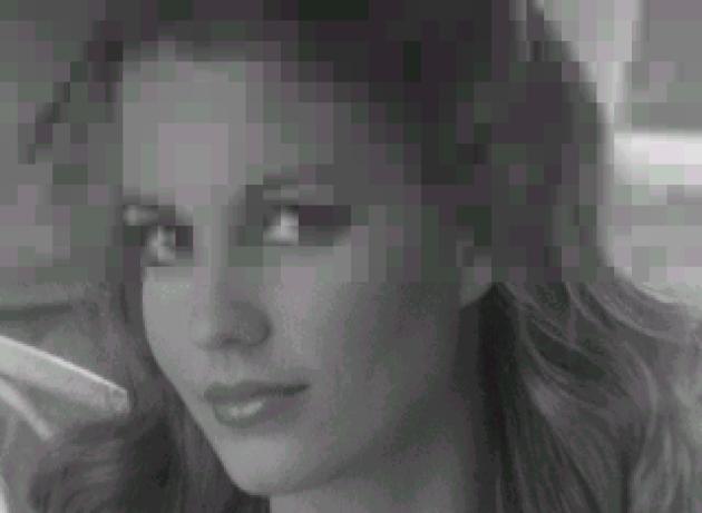
Upper Part:
Decompressed by Quality Factor->25
Lower Part:
Original Picture
Input
Bytes : 64000
Output
Bytes : 4170
Compression
ratio: 94%
RMS
Error : 6.6